One thing that I find really interesting and impressive about the APL language is the way it transforms traditional programming language into a succinct notation. Take for example the typical mean calculation. In traditional languages:

total = 0
    for i in x
        total = total + x
    mean = total / length of x

and in APL:

mean←(+/÷≢)x

The APL form is dense, but it summarises perfectly the intention. In signal processing there’s a similar way of transforming data from a visually obscure time domain into the frequency domain. In this post we will look at the Discrete Fourier Transform (DFT) and how it can be used to analyse data. We will be using the apl-sound-wave tools found on GitHub, so get yourself a copy if you want to follow along as you read.

Signal analysis using DFT

Without going into detail about the workings of the DFT, let’s just say that a signal in the time domain indicates the variation of amplitude over time. In the frequency domain however, we see variations of amplitude over frequencies. This means we can detect what frequencies are present in a signal and also the strength of each component. Let us start with a simple example: a single sine wave:

x4←#.SoundFX.Sine 4 0 1 100
      ]chart x4
      z4←|#.DSP.DFT x4
      ]chart z4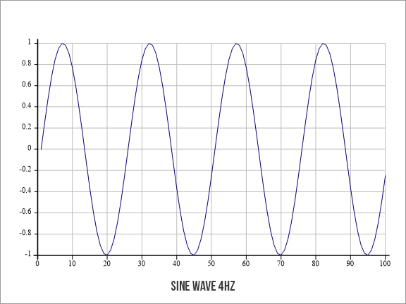

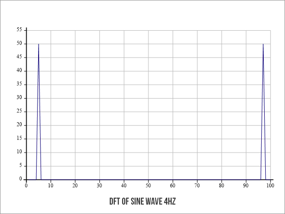
We generated a 4Hz wave with a duration of one second and a sample rate of 100Hz, so the first chart looks ok and we can see there are four peaks as expected. We then transform the samples into the frequency domain and plot the result (note that we are only interested in the amplitude and not phase, hence the vertical bar). The transform shows two peaks: one at the 4 marker and one at the 96 marker. The reason for this is that the transform always generates a mirrored curve due to the aliasing effect. Anything beyond the mid point (the Nyquist frequency) is simply a mirror of the first half. So can we ignore the second peak? Let’s generate another sine wave, this time with the frequency we can see in the transform chart, ie. 96Hz:

x96←#.SoundFX.Sine 96 0 1 100
      ]chart x4 x96
      z96←|#.DSP.DFT x96
      ]chart z96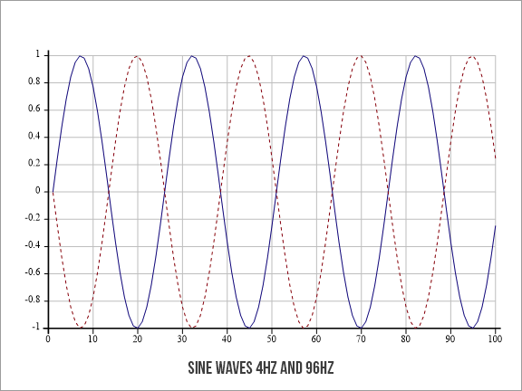

Hold on, isn’t that just an inverted 4Hz wave? Is the Sine generator broken?! Nope, this is the effect of undersampling which causes aliasing. To avoid this effect you must ensure that you sample the signal at least twice the highest frequency you are interested in.

In our first example we looked at a single, clean sine wave. In reality signals are complex with noise and overlaid frequencies. Let us simulate a noisy signal:

x20←#.SoundFX.Sine 20 0 1 100
      x20+←#.SoundFX.Noise 1 100
      ]chart x20
      z20←|#.DSP.DFT x20
      ]chart z20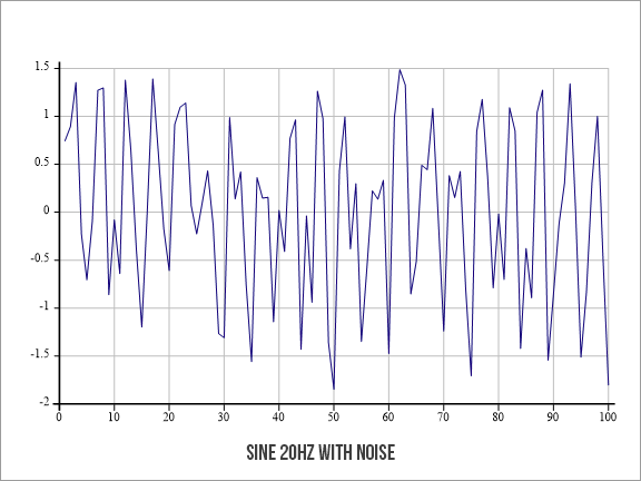

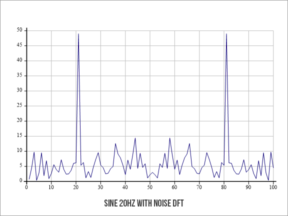
The noisy signal is barely visible in the first chart. We can see about 20 peaks, but it looks like pure noise. In the DFT however it is easy to detect that there’s a 20Hz signal in there. Finally, we step up the game by creating a mixture of three waves of increasing strength plus noise:

x234←2×#.SoundFX.Sine 20 0 1 100
      x234+←3×#.SoundFX.Sine 30 0 1 100
      x234+←4×#.SoundFX.Sine 40 0 1 100
      x234+←5×#.SoundFX.Noise 1 100
      ]chart x234
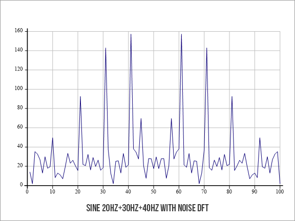
      z234←|#.DSP.DFT x234
      ]chart z234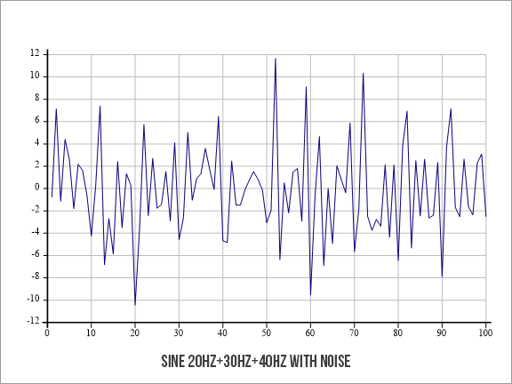

This is a good example of a noisy signal that is pretty much opaque to the naked eye and audibly unpleasant. You can play it with the command:

#.Sound.Play( #.SoundFX.Normalize x234) 100

Looking at the transform however, the three components are still distinguishable as well as their relative strengths. This way of analysing signals is critical in many systems. One of the most famous applications being touch dial phones using dual-tone multi-frequency signals (DTMF).

DTMF

We can generate DTMF tones and write them to file using the provided function like this:

sig←8192 #.SoundFX.DTMF '911'
      '.\dtmf911_8kHz.wav'#.Sound.Write sig 8192

That generates the three keys using a sample rate of 8192Hz (typical for phone line) and writes it out to a file. Similarly we can use the Read function to read a file into the ws:

wav←#.Sound.Read '.\dtmf911_8kHz.wav'
      sig sr←wav.(Samples SampleRate)

Provided that you apply the DFT to segments of the signal, you should be able to decode the signal and return the number that was called. As an exercise to the reader, write a DTMF decoder and see if you can identify the number called in the below audio sample.